Field note 001 / Mathematics on a GPU
Computation is also movement
An equation tells us what to compute. It leaves open how much information must move to compute it.
Two programs can evaluate the same equation and behave very differently on the same machine. That gap is interesting: it connects the mathematical description of a problem to the physical cost of solving it.
The first Mage investigation starts with five small operations. The question behind them is broader than kernel performance: what can the structure of a calculation tell us about how to organize the work?
Does the rewrite improve the work?
Start with a PyTorch expression, then give the same calculation to a custom Triton kernel and a Rust kernel built with cuda-oxide. The graphs show where the first rewrites improve the result and where they make it worse. Switch views to see why the choice of measurement matters.
RTX 4090 · FP32 · identical inputs
PyTorch baseline → first Triton and cuda-oxide Rust kernels

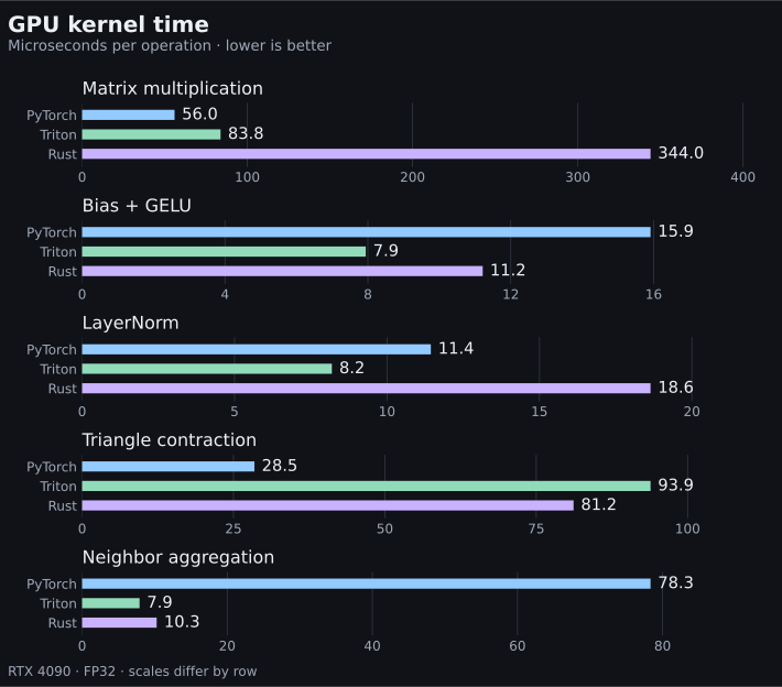
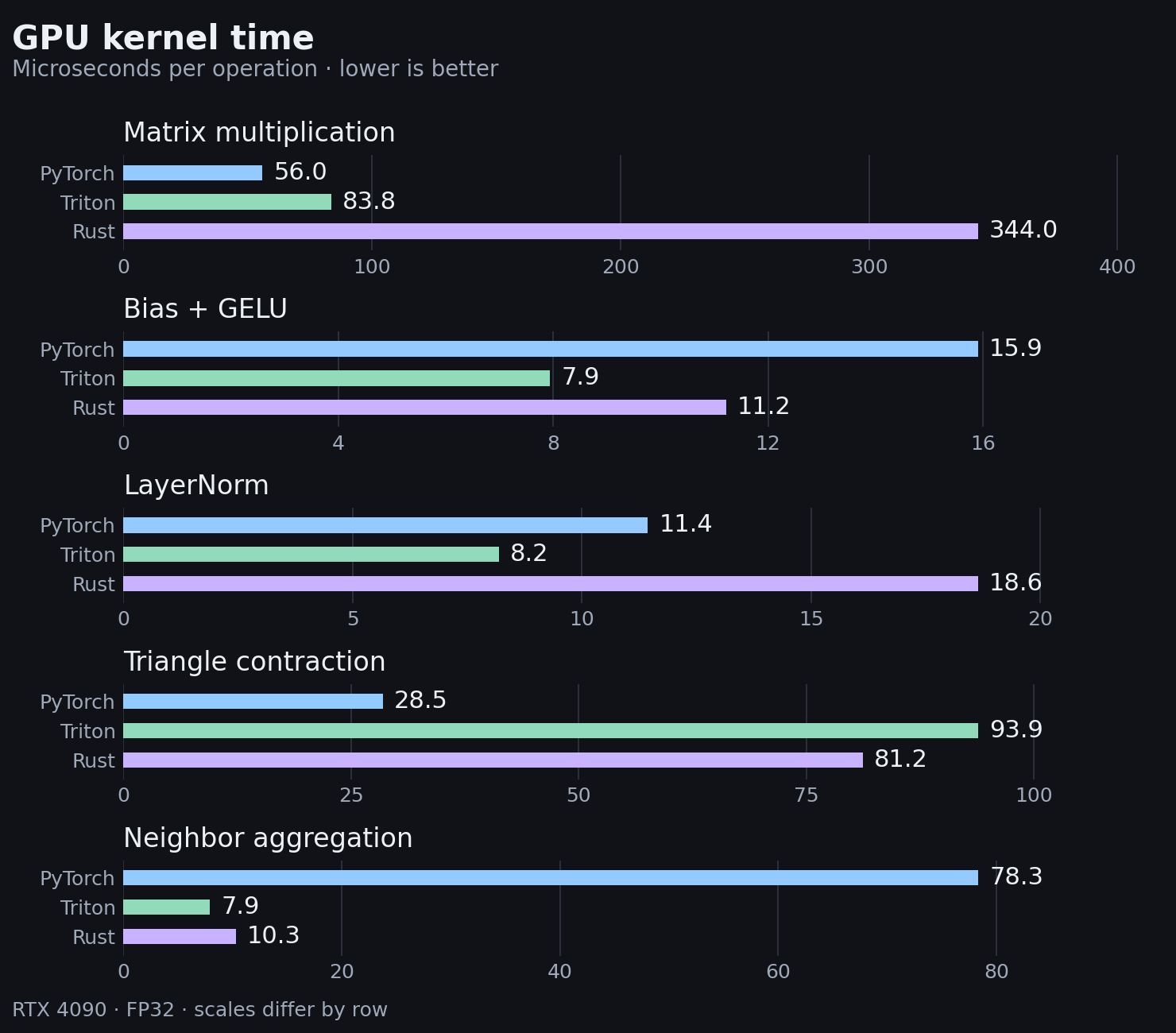
Time spent executing GPU kernels, summed per operation. A separate Nsight Systems capture of 100 iterations; gaps between launches are excluded. The WSL timestamp fallback has reduced precision.
Each row has its own scale. Compare implementations within a row.
Read the plotted values (µs)
| Operation | PyTorch | Triton | Rust |
|---|---|---|---|
| Matrix multiplication | 56.0 | 83.8 | 344.0 |
| Bias + GELU | 15.9 | 7.9 | 11.2 |
| LayerNorm | 11.4 | 8.2 | 18.6 |
| Triangle contraction | 28.5 | 93.9 | 81.2 |
| Neighbor aggregation | 78.3 | 7.9 | 10.3 |

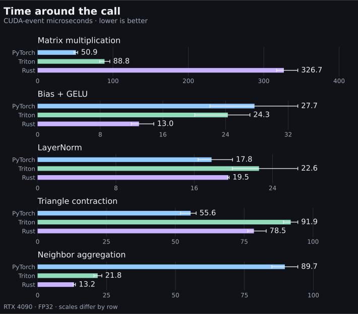
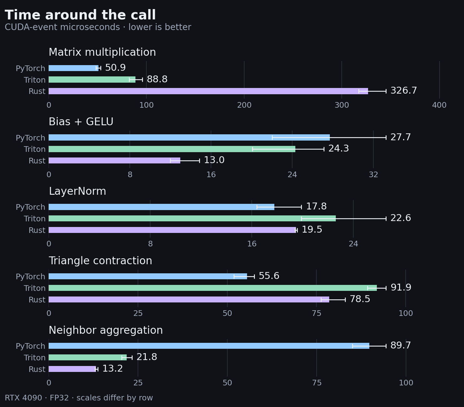
Mean of 300 warmed CUDA-event spans, collected in three rounds with rotating order. Whiskers show the range of the three round means, not a confidence interval. These spans can include gaps while the host submits work.
Each row has its own scale. Compare implementations within a row.
Read the plotted values (µs)
| Operation | PyTorch | Triton | Rust |
|---|---|---|---|
| Matrix multiplication | 50.9 | 88.8 | 326.7 |
| Bias + GELU | 27.7 | 24.3 | 13.0 |
| LayerNorm | 17.8 | 22.6 | 19.5 |
| Triangle contraction | 55.6 | 91.9 | 78.5 |
| Neighbor aggregation | 89.7 | 21.8 | 13.2 |

Captured launches divided by 100 iterations. Both custom implementations use one kernel per operation. Fewer launches help explain the result; they do not guarantee a faster kernel.
Each row has its own scale. Compare implementations within a row.
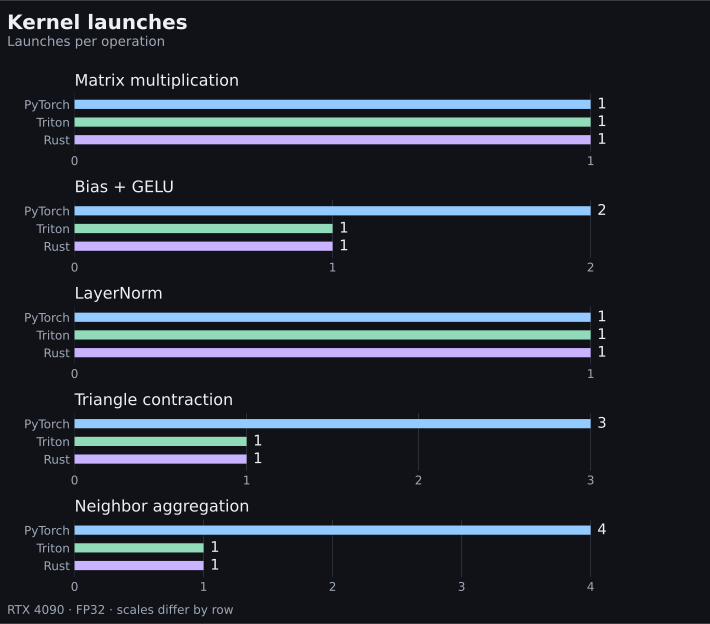
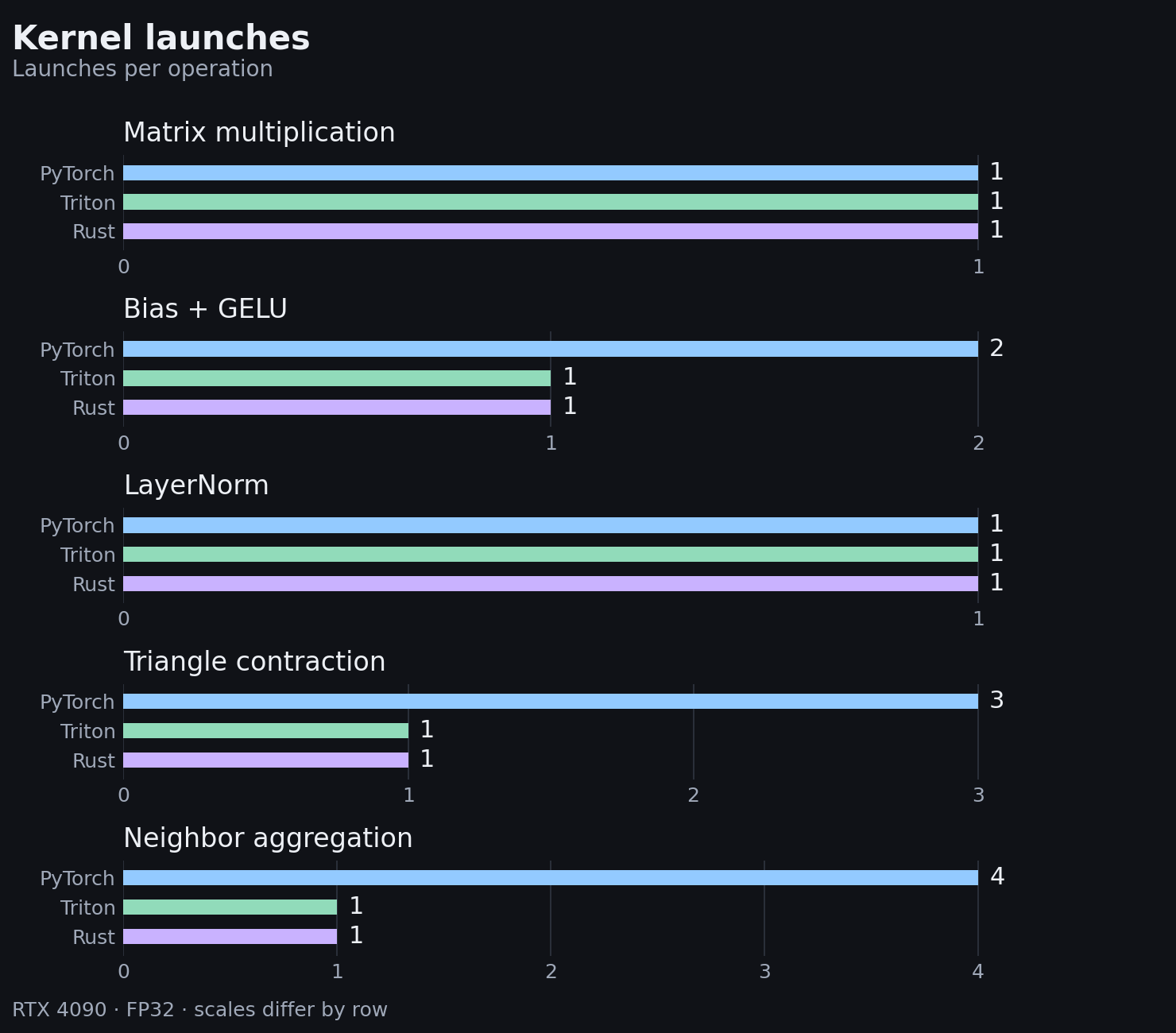
Read the plotted values
| Operation | PyTorch | Triton | Rust |
|---|---|---|---|
| Matrix multiplication | 1 | 1 | 1 |
| Bias + GELU | 2 | 1 | 1 |
| LayerNorm | 1 | 1 | 1 |
| Triangle contraction | 3 | 1 | 1 |
| Neighbor aggregation | 4 | 1 | 1 |
These are forward-only learning kernels at five fixed shapes, on one WSL workstation with unlocked clocks. Compilation, transfers, and service startup are excluded. This is a comparison of these implementations—not a production workload benchmark.

Both views in one figure. The top row is time inside the kernels; the bottom row is time around the call. Each column has its own scale, so implementations compare within a column. Bias + GELU is where the two views disagree.
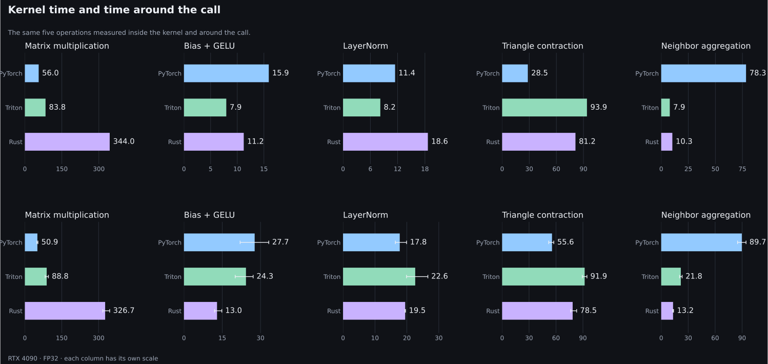
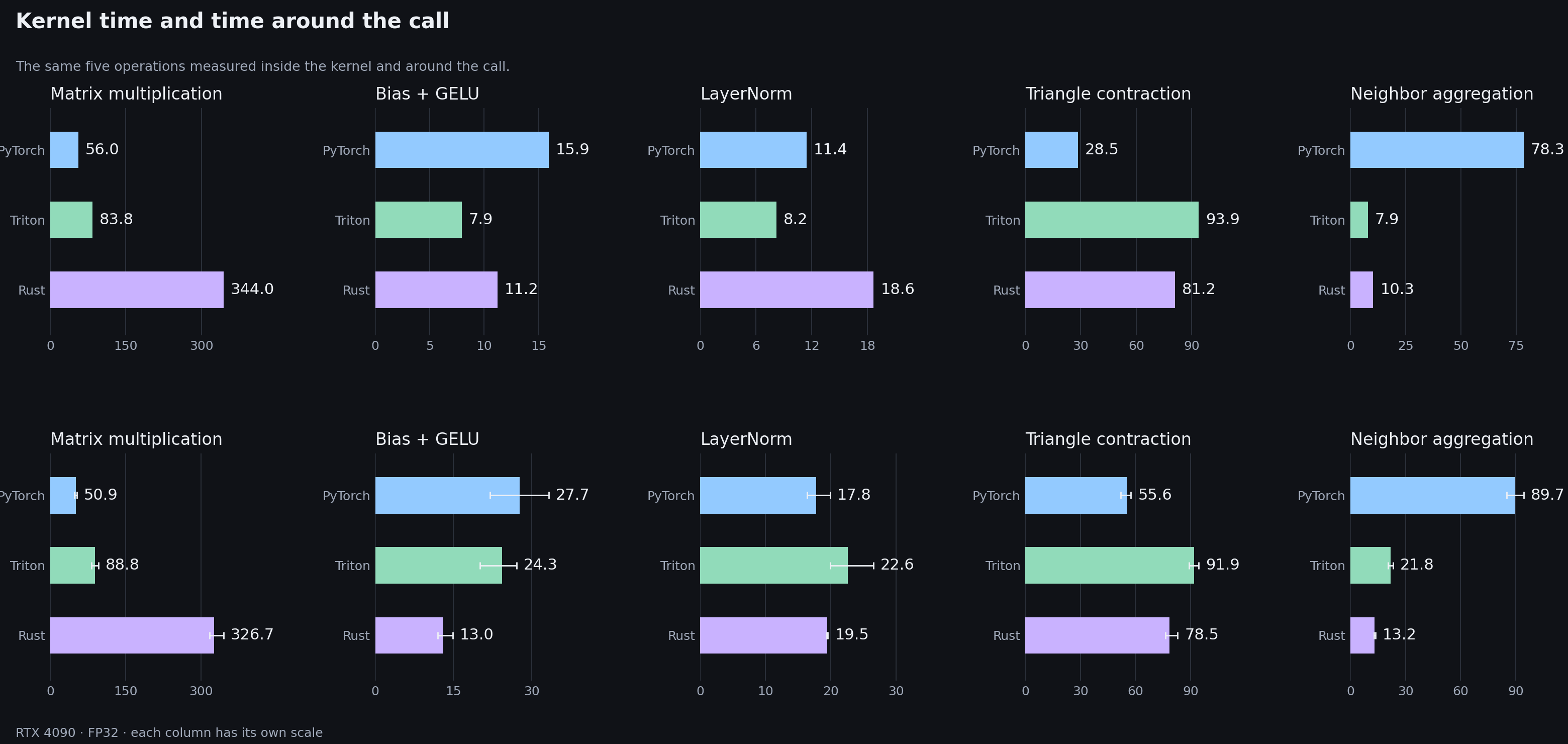
The surprising part is that the apparent winner can change with the measurement. For bias + GELU, Rust has the shorter event span around the call: 13.0 µs against Triton’s 24.3 µs. In the separate profile, Triton’s kernel itself takes 7.9 µs against Rust’s 11.2 µs. The launch path is part of the system we are measuring.
These are separate runs with different launch rhythms, so subtracting one number from another would not isolate Python overhead. They give us a better question to test: does the advantage survive when the kernel runs inside the actual application?
Reuse is hidden in the equation
Matrix multiplication looks like a collection of dot products:
\[C_{ij}=\sum_k A_{ik}B_{kj}.\]For one output, take a row from $A$, a column from $B$, multiply corresponding entries, and add. But neighboring outputs reuse much of that information. Move one column to the right and the row from $A$ is still the same.
A tile makes that reuse explicit. A 16 × 16 group of outputs can share two 16 × 16 input tiles. There are 512 distinct input values supporting 4,096 multiply-adds in one step along the shared dimension. The idea is to bring those values close to the threads and use them repeatedly.
This counts the structure of the calculation, not measured memory traffic: caches and the compiler also affect what reaches physical memory. The useful insight is that the equation contains an opportunity to reuse information, and the implementation can expose or obscure it.
That matters wherever repeated linear transformations dominate the work. A mathematical description becomes more useful when we can also see its dependencies.
A reduction chooses what survives
A sum turns many numbers into one. A dot product preserves one particular relationship between two vectors. A mean preserves a common level while discarding the individual deviations.
Layer normalization combines two reductions—a mean and a variance—to change how a row of features is represented. Subtracting the mean removes a shared offset. Dividing by a stabilized standard deviation controls the row’s overall scale. The relative pattern becomes easier to separate from that common level and magnitude.
There is a computational question inside that statistical idea: many threads can work independently on parts of a row, but eventually their partial answers must meet. Parallelism helps until information has to be combined. The arrangement of that meeting determines how much synchronization and movement the operation needs.
This is why learning reductions is useful beyond one neural-network layer. They recur in statistics, optimization, signal processing, and numerical simulation.
Local interactions become a larger structure
A weighted neighborhood sum is a simple way to describe influence:
\[y_i=\sum_{j\in\mathcal N(i)}w_{ij}x_j.\]Each entity receives information from its neighbors. The same pattern can describe a graph computation or form part of a model of interacting particles. The interpretation comes from what the nodes, edges, and weights represent; the algebra alone does not supply the physics.
A triangle contraction asks a related question about pairs. Instead of gathering directly from a neighbor, it combines two relationships through a shared third index:
\[O_{ijc}=\sum_k A_{ikc}B_{jkc}.\]The index $k$ is a meeting point. Reading the expression this way makes the connection to relational reasoning clearer than staring at nested loops. Protein-model-inspired tensor operations and graph-based materials models provide concrete places to explore these patterns. Our small kernels are primitives for studying the computation, not complete scientific models.
Compact notation is a beginning
Einsum notation helps name the relationships: which indices stay, which disappear, and which connect two quantities. It makes different-looking pieces of code easier to compare.
The next question is what the notation leaves unsaid. Where are the values stored? What gets reused? Which intermediate results must exist? Which can disappear?
The bias-and-GELU experiment is a small example of that last question. Bias changes each feature, and GELU applies a nonlinear transformation. A fused implementation can pass the intermediate value directly between the two steps. It evaluates the same intended operation with a different schedule for storage and execution.
What the first experiment taught us
All five Rust implementations matched the shared Python references in the tested cases. Their traces also made a useful distinction visible: one mathematical operation can become several kernel launches. The Python bias-and-GELU expression launched two kernels per iteration; the fused Rust version launched one.
That is an observation about these implementations, not a ranking of languages. The scalar Rust matrix multiply was substantially slower than the optimized Python library call. Reuse, instruction choice, launch overhead, and the quality of the implementation all matter.
The reason to keep measuring is to connect an idea to an explanation. A faster implementation is most useful to this investigation when we can say what changed and why it should help.
What would I use in production?
Keep the library where it already wins. PyTorch’s library-backed matrix multiplication and triangle expression beat both first custom versions in the GPU profiles. Replacing a mature implementation takes more than translating its equation into another language.
For a PyTorch workload, try compilation and targeted Triton fusion first. That is my starting recommendation for this project: Triton has the shortest measured GPU time for GELU, LayerNorm, and neighbor aggregation here, and PyTorch supports integrating Triton with its compiler and custom operators. These examples use fixed tiles; tuning and compiled execution still need their own comparison. Training also needs correct backward operations, which this experiment does not test.
For a Rust application, investigate the value of owning the whole launch path. Native integration, explicit memory ownership, and control over execution can justify the work. A shorter event span in this harness is a reason to investigate, not enough to ship a replacement. cuda-oxide describes itself as an experimental alpha compiler, so a production candidate needs a pinned toolchain, a fallback, and validation on the deployment hardware.
The decision belongs to the whole workload. If a kernel accounts for 20% of a request, making it twice as fast improves the full request by only about 11%, assuming the rest is unchanged. The next useful experiment should therefore measure an actual model or service: representative shapes and precision, batching, transfers, throughput, and tail latency. That is where a faster kernel earns its place.
Measurements and reproduction in GitHub · Why this investigation exists
Further connections: V-JEPA 2, AlphaFold 3, and MACE.