Journal / 10 September 2026

The male CNS, as arrays

The complete male fruit fly central nervous system — 166,700 neurons, 11,710 types, 45.6 million pre-synaptic sites — is public, fits on one workstation, and reduces to a 929,735-edge graph between types. That is small enough to compute on a GPU and specific enough to steer a robot with.

By Superposition · Updated 11 September 2026

The four spots are the four cross-sex classes of cell type, opacity set by the log of each class's count: isomorphic, dimorphic, male-specific, female-specific.

Field: Paper Shaders mesh gradient (Apache-2.0), palette and weights from this post.

The claim. The whole central nervous system of a male fruit fly is now public data — 166,700 neurons, 11,710 cell types, 45.6 million pre-synaptic sites — and it is small enough to hold on one workstation. Reduce it to the graph between cell types and it becomes 929,735 edges over 11,687 types, which is a graph a GPU can sweep thousands of times while you wait. What is computable is therefore no longer “where does this neuron go” but “what happens to the circuit if this class of neuron is rewired” — and the classes that differ between the sexes are an enumerable list: 138 dimorphic and 289 male-specific types. That list is the thing worth computing on, and it is the thing that can be handed to a robot as a cost.

This post is a map and a plan, not a result. Every number below is the dataset’s; nothing on it has been computed yet, and the last section says exactly where the plan stops.

What the map is

One adult male, all of it: central brain, both optic lobes, and the ventral nerve cord in a single seamless volume — the first complete male CNS connectome, published in Cell in 2026 with a preprint in 2025.

Quantity	Value	Where it comes from
Neurons	166,700	Berg et al. 2026, Cell
Cell types	11,710	same
Pre-synaptic sites (T-bars)	45,656,140	Neuprint_Meta.csv, male-cns:v1.0
Post-synaptic sites	311,833,243	same
Segment-to-segment edges	151,856,684	connectome-weights export
Neuron-to-neuron edges with valid superclasses	25,563,426	the paper’s own notebook
Edges at weight ≥ 5	6,237,402	same
Type-to-type edges	929,735	same, aggregated over 11,687 types

All eight values are quoted; the last line is the one that matters here.

The type-level graph is the useful scale. Written as a dense matrix it would be

\[\frac{929{,}735}{11{,}687^{2}} \;\approx\; 6.8 \times 10^{-6}\]

that is, about seven entries in a million — sparse enough to store as a list, small enough to hold several copies of, which is what makes sweeps affordable.

The sex comparison is where the numbers get sharp. Against the female FlyWire connectome, the types split into 8,069 isomorphic, 138 dimorphic, 289 male-specific and 71 female-specific. Put differently: roughly 95% of cells are shared, about 12% of neurons in the male brain show wiring differences against fewer than 3% in the female brain, and the male-specific and dimorphic types together are a few hundred names — small enough to enumerate by hand, large enough to be a real circuit.

How it gets onto one machine

Two doors, and they are not equivalent:

Python, for arrays. neuprint-python talks to the server at neuprint.janelia.org and returns pandas or Arrow tables; navis and navis-flybrains handle skeletons, meshes and coordinate transforms. This is the door for anyone who wants the connectivity as arrays and a GPU underneath it.

R, for the annotation ecosystem. neuprintr plus malevnc (the nerve-cord subset, MANC: about 23,000 neurons, 10 million pre-synaptic sites, 74 million post-synaptic densities) or malecns (the whole CNS). malecns is, in its own words, “a very thin wrapper around the malevnc package”. This is the door for Clio annotations and template-brain registration across light-level templates.

The bulk data sits on a public Google Cloud bucket, and this is the part that decides what kind of work is possible:

Export	Size	Rows
syn-points (pre + post)	13.061 GB	357,489,383
syn-partners (one row per post-synaptic contact)	6.777 GB	311,833,243
connectome-weights (segment to segment)	1.051 GB	151,856,684
Neuprint_Neurons (all segments)	4.649 GB	88,682,452

Row counts are read from each file’s Arrow footer, and the first two check out against the dataset’s own metadata: $45{,}656{,}140 + 311{,}833{,}243 = 357{,}489{,}383$.

That is a couple of hundred gigabytes of local disk at most, and the connectivity itself — the 1.051 GB export — is a file you can open in a notebook.

Four things make the wrangling harder than the download, and all four are worth knowing before writing code:

• Identity is per segment, not per neuron. The Neuprint_Neurons export has 88.7 million rows, because it also carries untraced fragments. The neuron count comes from the annotation table (211,577 rows with curated annotation) and from the status field, not from the row count.
• A pre-synaptic site is not a connection. One T-bar can contact several partners, so connections exceed pre-synaptic sites; weight on the ConnectsTo edge is the count of contacts. Connections and synapses are different quantities and the press numbers mix them.
• Sign is inferred. There is no excitatory/inhibitory column. There are predicted neurotransmitter probabilities per neuron and per T-bar — ACh, GABA, glutamate, dopamine, octopamine, serotonin, histamine, tyramine — and the sign is a reading of those.
• The join keys are the point. Each type can carry flywireType, mancType, hemibrainType, vfbId and a itoleeHl hemilineage; 8,137 of the 11,751 type entries in the explorer carry a FlyWire type. Cross-dataset work is a join on those columns, and where they are empty the join is simply unavailable.

What the GPU is actually for

Not size. The adjacency is 1 GB, and any laptop holds that. The GPU is for repetition: every question worth asking about a circuit is a null test — how surprising is this many connections between these two types; what survives if these 289 types are rewired at random; which dimorphic types are dimorphic in a structured way rather than by drift. Each of those is a full pass over the edge list, and there are thousands of them.

The primitive is one we have already measured. Neighbour aggregation over a CSR edge list — a rowptr array, an indices array, a weights array, one output row per input row — is exactly the shape of a connectome statistic, and on the RTX 4090 it runs at 7.06 µs over 65,536 edges after the load-widening change (Triton’s kernel, 5.97 µs, is still ahead). The type graph is about fourteen times larger, so one statistical sweep is on the order of a tenth of a millisecond; ten thousand permutations then cost seconds, not hours, and that is the whole argument for the card.

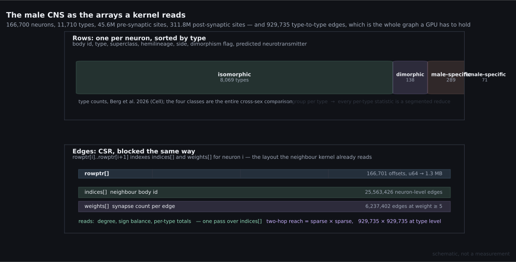
The connectome as the two arrays a kernel actually reads. Sorting by type is what makes the per-type statistics a segmented reduce instead of a sort inside the kernel. Download the SVG.

Three kernels cover most of it: a degree and sign census (one pass, per-type segmented reduce), a two-hop reach — sparse × sparse, $929{,}735 \times 929{,}735$ at type level, which is how you ask “what does this class touch through one intermediate” — and permutation tests, the same census run across shuffled adjacency, where the GPU’s job is to run many tiny independent versions of the same kernel rather than one large one.

How it drives

The loop it feeds already exists, in two repositories.

leash is a safety-gated Rust robotics runtime: CLI, HTTP and MCP control over simulation, replay and physical hardware, with the safety authority — authorization, approval, deadman, freshness, collision, distance, stop, latching E-stop — held by the runtime and not by the caller. Its compute surface is exactly what this needs: a bounded, authenticated, advisory job API (POST /compute/jobs, results capped at 1 MiB, at most two concurrent, deadlines up to 120 seconds) whose own documentation states that compute results “cannot authorize or refresh motor output”. The leash-cuda crate owns the on-robot CUDA contract: a checked-in fatbin for the Jetson Orin NX (SM 8.7, CUDA 12.9, SHA-256 recorded in a manifest, six kernels each compared against a CPU oracle), built deliberately rather than compiled at startup.

qualia is the runtime that carries the higher-order state, and its planner speaks a frozen contract: plan_path over a local socket as newline-delimited JSON, taking a start pose, a goal pose, an occupancy grid, constraints — and a belief_risk block of two floats:

\[\text{path\_cost} \;\mathrel{+}=\; \big(\text{uncertainty\_weight} \times 12 \;+\; \text{novelty} \times 4\big) \times \text{resolution}_m\]

That is the seam. The planner today is grid-only — A* or uniform cost over a 2D occupancy grid — so a connectome does not become the planner. It becomes a prior on the cost: a table saying where the male-specific and dimorphic circuitry is involved, which the planner already knows how to price in, with the evidence attached and the authority left where it is.

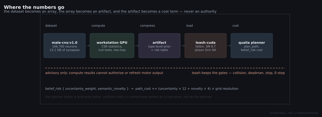
The path from a connectome to a robot's cost function. The dashed rule is the important line in the diagram: the numbers are advisory, and the gates that can stop a motor stay with leash. Download the SVG.

What this does not establish

Nothing on this page has been computed. The dataset numbers are quoted from the paper, the release metadata and the exports; the graph sizes are read from file footers; the kernel time is from the earlier profiling session and is a neighbour-aggregation kernel on synthetic edges, not on this data. The plan — map, compute, price — is a plan.

Beyond that, four things are open or unresolved and none of them are small:

• The step from structure to a cost is the research problem. Knowing that 289 types are male-specific does not say what a robot should do differently. Nothing here identifies which of those types, if any, corresponds to a navigational decision; that mapping would have to be earned.
• Version and count discrepancies. The paper says 11,710 types, the v1.0 explorer says 11,751, and the preprint said 11,691; the explorer’s catalog sums to 164,838 cells against the paper’s 166,700 neurons. Two different dataset UUIDs circulate (one in the neuprint metadata, one in the explorer). I have not resolved any of these.
• The press figure is not the table figure. “125 million synaptic connections” does not match the 311.8 M post-synaptic sites or the 151.9 M segment-to-segment edges; the arithmetic that reconciles them is not stated in any source I found, and I have not asserted one.
• Sign, and the parts of the nervous system the plan ignores. Excitatory/inhibitory is inferred from neurotransmitter prediction, not measured. Neuromodulation, gap junctions, and everything that is not a chemical synapse are outside the edge list; so is the animal, since a connectome recorded from one male fly is a single sample of a species.

The download page has the exports; the paper and its preprint have the biology; malecns and 2025malecns are the two access paths this post uses; leash is where the numbers would land.